Introduction

The goal of this project is to design and implement a control system for an instrumented ebike used in bicycle handling experimentation. To achieve this, a basic unity feedback control architecture (Figure 1) is employed.

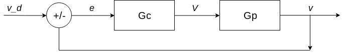
Figure 1. Control architecture where e is the error between the actual speed v of the ebike and the desired speed, vd, and V is the DC input voltage to the ebike plant model. Gc and Gp represent the controller and plant model respectively.

The goal of the controller is to track a setpoint speed, within +/- 0.10 m/s, set by the rider. To achieve this, a PID controller was tuned using MATLAB’s Control System Toolbox. The ebike plant model was derived using first principles and grey box system identification.

Modeling the eBike From First Principles

The dynamics of the ebike powertrain and the vehicle itself can be modeled from first principles. The powertrain of the ebike consists of a standard ebike conversion kit motor controller and a brushless 3 phase direct drive induction motor mounted to the rear hub of the bike. A simple diagram of the ebike drivetrain is shown below in Figure 2.

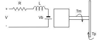
Figure 2. Diagram of the drivetrain circuit and dynamics.

In Figure 2, the induction motor is approximated by a model of a DC motor circuit with resistance \(R\), inductance \(L\) and back emf \(V_b\). The torques \(T_m\) and \(T_p\) acting on the motor shaft correspond to motor torque and wheel propulsion torque respectively. The rotational dynamics of the drivetrain are defined by Euler’s rotation equation.

A simple equation of motion for the bicycle, modeled as a point mass, is derived using Newton’s 2nd Law of Motion in the horizontal direction [Wilson].

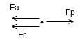
Figure 3. Free body diagram of the bicycle modeled as a point mass. Fa, Fr and Fp are the aerodynamic drag, rolling resistance and propulsive forces respectively.

Together, the vehicle and drivetrain dynamics of the ebike can be shown in a state space representation with state variables \(i(t)\) and \(x(t)\) as seen below.

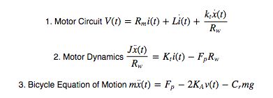
From the state space representation, a transfer function from input DC voltage \(V\) to output speed \(v\) is formed:

This plant model is a second order transfer function relating an applied DC voltage input to the ebike’s motor controller to the output speed of the ebike. This model represents an approximation of the true plant model of the ebike. To get a more accurate plant model, a grey box system identification procedure based on measured time response data from the ebike was used.

Performing System Identification From Experimental Data

To begin the process of system identification, the values of the ebike drivetrain model parameters and bicycle drag and tire rolling resistance coefficients were initialized using reasonable approximations found from internet searches, previous knowledge of the instrumented ebike [Moore] and textbook resources [Wilson].

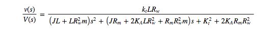
In MATLAB, a nonlinear least-squares solver was used to optimize the constants in the derived plant model of the ebike to match a speed time response measured from the instrumented ebike. Figure 4, below, shows the curve fitting result.

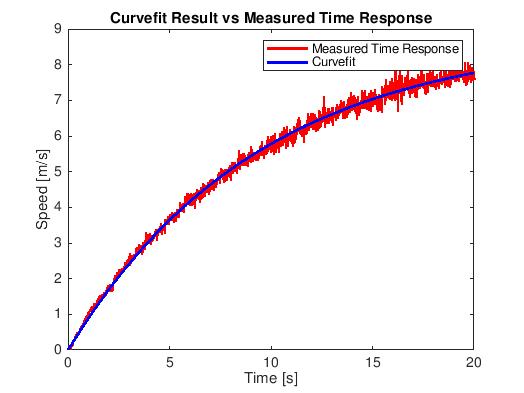
Figure 4. Result of the least-squares curve fitting.

Figure 4 shows that the plant model of ebike was reasonably identified using the least-squares curve fitting method. The resulting ebike plant model is:

Controller Design in MATLAB

With the plant model of the ebike identified, a PID controller (kp = 68.5, ki = 106, kd = 1.44) was tuned for zero steady state error and reasonable transient behavior using MATLAB’s Control System Toolbox.

The closed loop step response (Figure 5) shows that the controller meets the design goals with zero steady state error, a settling time of 1.56s, and an overshoot percentage of 10.45%.

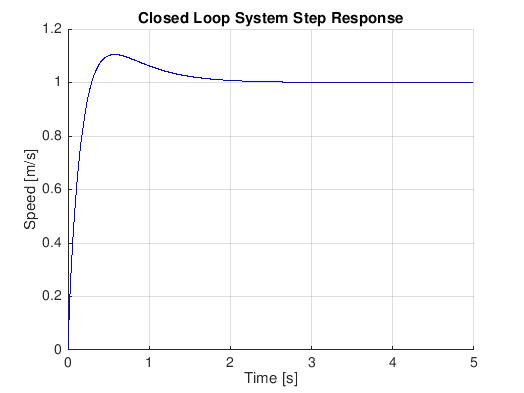
Figure 5. Closed Loop System Step Response.

Evaluation of Controller Robustness

MATLAB’s Robust Control Toolbox was used to test the robustness of the closed loop system with regards to uncertainties in the coefficients of the identified ebike plant model. The constants in the derived ebike plant model were lumped together forming the following simplified plant model:

The constants \(a\), \(b\), \(c\), and \(d\) in the above transfer function were defined in MATLAB as real-uncertain parameters with varying percentage based uncertainties about their nominal values. The nominal values of each coefficient were taken from the result of the system identification step of the controller design process. Figure 6, below, shows the nominal closed loop and open loop system step response with 20 random samples of the uncertain plant model defined by the uncertain coefficients.

Figure 6. Step response of the nominal closed loop system with 20 random samples of the uncertain closed loop step response superimposed on the plot.

Figure 6 shows that the closed loop system is reasonably robust despite uncertainty in the plant model. Having this robustness in the control system means that small changes in the dynamics of the ebike will not cause the controller to have undesirable performance.

Conclusion

A simple PID controller used in a unity feedback control architecture was designed to reduce the steady state error and improve the transient performance of the speed time response of an instrumented ebike. Using grey box system identification, the plant model of the ebike was identified and used in the controller design. A PID tuner app was used to tune the controller constants to achieve zero steady state gain and favorable transient behavior. Finally, the robustness of the controller was tested by simulating uncertainties in the closed loop system.

The next step in the project is to take the continuous time PID controller and implement it digitally on the instrumented ebike. Stay tuned for part two: Implementing a PID Controller on an Instrumented Ebike.

References