
- Fri 27 October 2023
- research
- Jason K. Moore
- #sympy, #czi, #biomechanics, #multibody dynamics, #open source software, #muscles, #optimal control, #bicycle, #skateboard, #code generation
 |
Introduction
We were awarded a two year grant from CZI to improve SymPy. There were three work packages led by each of the three co-principal investigators:
- Improve SymPy's Documentation (Aaron Meuer, Quantsight)
- Improve SymPy's Performance (Oscar Benjamin, University of Bristol)
- Improve SymPy's Code Generation for Biomechanical Modeling (Jason K. Moore, Delft University of Technology)
We were in charge of the last work package and hired Dr. Sam Brockie to work on the project as a postdoctoral researcher. Jan Heinen and Timo Stienstra worked on the project through their TU Delft MSc degrees under the supervision of Sam and Jason.
Our overarching goal is to use SymPy to generate symbolic dynamical models of biomechanical systems, i.e. multibody systems actuated by muscles. This involves formulating the Newton-Euler equations of motion, possibly with additional kinematic constraints, and the differential equations that describe the relationship between neurological excitation and generated muscles forces.
We selected a complex human-machine system as a benchmark problem to motivate our work: the bicycle and its rider. The nonlinear and linear equations of motion of a riderless bicycle have traditionally been a very challenging system to derive correctly in full symbolic form (see [BasuMandal2007] and [Meijaard2007] for background). Including a model of a human rider with muscle-driven joints increases the model's complexity even further. This model is made up of millions of arithmetic and transcendental operations, making it a challenging system to differentiate and evaluate efficiently. We want SymPy to be able to handle models of this complexity with ease. To test SymPy's ability to correctly derive, differentiate, and evaluate the bicycle-rider's governing equations, we choose to formulate and solve a trajectory optimization problem via direct collocation. We knew that this bicycle-rider optimal control problem would test SymPy's limits, forcing us to make significant improvements to SymPy's code generation features. To do this, we worked on numerous areas in SymPy and downstream packages to reach this goal.
General Improvements to SymPy Mechanics
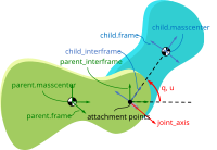
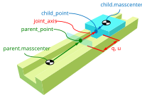
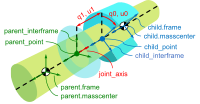
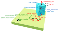
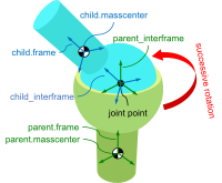
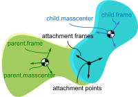
Joints Package
Timo Stienstra began working on this project through a 2022 Google Summer of Code internship where he improved the SymPy Mechanics joints modules with documentation improvements, by reworking the fundamental definition of a joint, and adding new cylindrical, planar, and spherical joints. These were key early updates to enable the joints package's use in constructing a bicycle-rider model. See the details of Timo's work in his GSoC Report. This project led Timo to do a TU Delft Biomechanical Design MSc project on bicycle-rider modeling using SymPy.
 |
 |
 |
 |
 |
 |
Symbolic Solutions to Linear Equations
Kane's Method relies on solving three sets of linear equations:
- putting the kinematical differential equations in explicit form \(\dot{\mathbf{q}} = \mathbf{M}_k^{-1}\left(\mathbf{u} + \mathbf{f}_k\right)\)
- putting the dynamical differential equations in explicit form \(\dot{\mathbf{u}} = \mathbf{M}_d^{-1}\mathbf{f}_d\)
- solving the dependent generalized speeds in terms of the independent generalized speeds \(\mathbf{u}_r = \mathbf{A}_r^{-1}(\mathbf{A}_s\mathbf{u}_s + \mathbf{f}_{rs})\)
If these equations are symbolic, it is mostly impossible to determine if an entry is zero when pivoting in Gaussian elimination making the solutions susceptible to divide-by-zero operations for ranges of numerical values for the variables involved.
There are four ways, it seems, to deal with this:
- select the generalized coordinates, generalized speeds, and constants such that divide-by-zero cannot occur for the numerical values of interest
- select symbolic Gaussian elimination algorithms that do not put the solutions in a form that has divide-by-zero for the numerical values of interest
- use a zero-division free linear solve algorithm
- defer the linear solves to numerical algorithms
1. Choice of Generalized Coordinates and Speeds
The choice of generalized coordinates and generalized speeds changes which entries in the linear coefficient matrix can be zero for specific values of the coordinates and speeds. It may be possible to avoid divide-by-zero with careful selection of the variables when defining the kinematics of the specific problem. But this will require unique solutions for every model.
2. Alternative Symbolic Solvers
In 2014, we switched to using LUsolve() for all of the linear solves in SymPy Mechanics in PR 7581, which resulted in an unnoticed regression of divide-by-zero issues for complex problems. This change broke the crucial test_kane3.py as well as the corresponding documentation page that solved the linear Carvallo-Whipple bicycle model to a machine precision match against published benchmarks. This bug has hounded us for 9 years (see https://github.com/pydy/pydy/pull/122 and https://github.com/sympy/sympy/issues/9641).
Timo discovered the fundamental divide-by-zero issue after much sleuthing and discussion. He then introduced a new linear solver that uses Cramer's rule, which can eliminate divide-by-zero operations in many cases. We then added support to KanesMethod() and Linearizer() for using linear solvers other than LUSolve() including the new Cramer's rule-based solver as an option. With this we closed the 9 year old bug and allowed our base bicycle model to build both in non-linear and linear forms. The new Cramer solve method for matrices was introduced in https://github.com/sympy/sympy/pull/25179.
3. Division-free Linear Solves
There are division-free algorithms that can be used in solving linear systems, but the complexity of the resulting equations grows considerably, for example see [Bird2011].
4. Delayed Numerical Solves
It would be helpful if we could delay linear solves to the numerical evaluation, so that pivot points can managed by LAPACK's solvers. To do so, we would need to be able to use the results of a linear solve like any other symbol without symbolically evaluating the linear solve operation. The following SymPy code almost works as desired:
from sympy import MatrixSymbol, Inverse, lambdify

A = MatrixSymbol('A', 2, 2)
b = MatrixSymbol('b', 2, 1)
x = Inverse(A) @ b
result = x[0, 0] + x[1, 0]
eval_result = lambdify((A, b), result)
The above works but the inverse and matrix multiplication are evaluated symbolically when called, as can be seen in the generated function:
>>> help(eval_result)
...
Source code:

def _lambdifygenerated(A, b):
    return A[0, 0]*b[1, 0]/(A[0, 0]*A[1, 1] - A[0, 1]*A[1, 0]) - A[0, 1]*b[1, 0]/(A[0, 0]*A[1, 1] - A[0, 1]*A[1, 0]) - A[1, 0]*b[0, 0]/(A[0, 0]*A[1, 1] - A[0, 1]*A[1, 0]) + A[1, 1]*b[0, 0]/(A[0, 0]*A[1, 1] - A[0, 1]*A[1, 0])
...
Instead, we'd like lambdify() to generate code that looks more like:
def eval_result(A, b):
   x = numpy.linalg.solve(A, b)
   return x[0, 0] + x[1, 0]
which allows NumPy (or actually LAPACK) to use the appropriate algorithm given the numerical values used for A and b. The expression Inverse(A) @ b would need to remain unevaluated for code generation to properly handle it. In SymPy, there is a MatrixSolve() code generation node that acts as an unevaluated linear equation solver and works as desired with lambdify():
>>> from sympy.codegen.matrix_nodes import MatrixSolve
>>> x = MatrixSolve(A, b)
>>> eval_x = lambdify((A, b), x)
>>> help(eval_x)
...
Source code:

def _lambdifygenerated(A, b):
    return solve(A, b)
...
But MatrixSolve() does not support indexing the solution:
>>> result = x[0, 0] + x[1, 0]
---------------------------------------------------------------------------
NotImplementedError                       Traceback (most recent call last)
Cell In[8], line 1
----> 1 result = x[0, 0] + x[1, 0]

File ~/miniconda/lib/python3.9/site-packages/sympy/matrices/expressions/matexpr.py:300, in MatrixExpr.__getitem__(self, key)
    298 i, j = _sympify(i), _sympify(j)
    299 if self.valid_index(i, j) != False:
--> 300     return self._entry(i, j)
    301 else:
    302     raise IndexError("Invalid indices (%s, %s)" % (i, j))

File ~/miniconda/lib/python3.9/site-packages/sympy/matrices/expressions/matexpr.py:243, in MatrixExpr._entry(self, i, j, **kwargs)
    242 def _entry(self, i, j, **kwargs):
--> 243     raise NotImplementedError(
    244         "Indexing not implemented for %s" % self.__class__.__name__)

NotImplementedError: Indexing not implemented for MatrixSolve
Timo has an open pull request that uses BlockMatrix() with MatrixSolve() for the solution of dependent speeds in KanesMethod, that can at least give this delayed solve with lambdify(modules='NumPy'), see https://github.com/sympy/sympy/pull/24916.
Inertia, Loads, Actuators
We introduced three new helper classes to extend the functionality of inertia and loads beyond that of simply dyadics and vectors: Inertia(), Force(), and Torque(). The inertia object lets you associate a dyadic with a point, to completely define inertia for a rigid body, particle, or collection of them. Force and Torque are named tuples that associate a vector and point and a vector and a frame, respectively.
We have introduced an actuator module that has classes that describe the equal and opposite pair of forces or torques and force actuators can operate along a pathway, generating resultant forces on points that lie along the pathway. We included a linear spring and damper as example actuators. The pathways are located in the new pathway module.
These new objects provide core building blocks for developing musculotendon actuators and managing a full multibody system.
System Class
Timo developed a new System() class that manages all the information about a multibody system (coordinates, joints, bodies, constraints, etc.) and can generate the equations of motion from the high level description of the system without having to manually write the mathematical equations. This approach generally reduces the amount of code needed to generate the equations for complex systems. See the Four-bar Linkage example to get an idea of how it works.
Introducing SymPy Biomechanics
We have developed a substantial new sub-package, sympy.physics.biomechanics, that enables including musculotendon force actuators in multibody dynamics models created with sympy.physics.mechanics. biomechanics contains these primary modules:
- curve.py: contains classes that represent mathematical functional relationships between the time-varying muscle-tendon length, velocity, and force
- activation.py: contains classes that manage the excitation to activation dynamics
- musculotendon.py: contains classes that represent complete musculotendon models with one reference implementation from [DeGroote2016]
A full explanation of this package and the modules can be found in the new Introduction to Biomechanical Modeling tutorial. We demonstrate the package on a non-trivial biomechanical system in the new Biomechanical Model Example tutorial.
 |
 |
Code Generation Improvements
The function lambdify() is the primary interface for converting SymPy expressions into NumPy-powered Python functions for numerical evaluation. lambdify() relies on SymPy's code generation to generate the appropriate Python code. lambdify() has not been able to handle large mechanics models in the past. We proposed adding common sub-expression elimination (CSE) support to help with that. Support for the cse() function was added to lambdify() just before we started the CZI work in https://github.com/sympy/sympy/pull/21546. Here is an example that demonstrates some of the speed improvements:
from sympy import count_ops, lambdify
from sympy.physics.mechanics import find_dynamicsymbols, dynamicsymbols
from sympy.physics.mechanics.models import n_link_pendulum_on_cart
import numpy as np
Generating the equations of motion with KanesMethod will be faster for some models in the next release of SymPy due to Pull Request 24792. This shows the speed in SymPy 1.11.1:
In [1]: %time kane = n_link_pendulum_on_cart(n=14)
CPU times: user 7.45 s, sys: 3.69 ms, total: 7.46 s
Wall time: 7.47 s
and the same in the tip of the master branch (1.13.dev0):
In [1]: %time kane = n_link_pendulum_on_cart(n=14)
CPU times: user 4.85 s, sys: 3.81 ms, total: 4.85 s
Wall time: 4.85 s
large_expr = kane.mass_matrix_full @ kane.forcing_full
x = list(find_dynamicsymbols(large_expr))
p = list(large_expr.free_symbols)
p.remove(dynamicsymbols._t)
x_vals, p_vals  = np.random.random(len(x)), np.random.random(len(p))
These expressions have almost 300 thousand operations:
In [1]: count_ops(large_expr)
Out[1]: 282836
In SymPy 1.12, lambdifying large expressions will take at least half the time as prior versions because there is wasted time printing the full expression to the docstring. Sam sped up lambdify's code generation by disabling the docstring generation for large expressions in Pull Request 24754. Note that lambdifying expressions is also faster with cse=True. Here is the timing in SymPy 1.11.1:
In [1]: %time f_without_cse = lambdify((x, p), large_expr)
CPU times: user 29.4 s, sys: 91.3 ms, total: 29.5 s
Wall time: 29.5 s

In [2]: %time f_with_cse = lambdify((x, p), large_expr, cse=True)
CPU times: user 14.5 s, sys: 15.8 ms, total: 14.5 s
Wall time: 14.5 s
and then the same in SymPy 1.12:
In [1]: %time f_without_cse = lambdify((x, p), large_expr)
CPU times: user 17.9 s, sys: 68.4 ms, total: 18 s
Wall time: 18 s

In [2]: %time f_with_cse = lambdify((x, p), large_expr, cse=True)
CPU times: user 2.77 s, sys: 7.93 ms, total: 2.77 s
Wall time: 2.77 s
Using cse=True with lambdify(), results in significantly faster numerical evaluation:
In [2]: %timeit f_without_cse(x_vals, p_vals)
40.7 ms ± 824 µs per loop (mean ± std. dev. of 7 runs, 10 loops each)

In [3]: %timeit f_with_cse(x_vals, p_vals)
264 µs ± 7.37 µs per loop (mean ± std. dev. of 7 runs, 1,000 loops each)
For this example, the CSE version is 154X faster at execution.
Modeling and Optimal Control Uses
As explained in the introduction, our goal is to make SymPy capable of deriving computationally efficient neuromuscular driven multibody models. One use case for these models is solving optimal control problems, which benefit greatly from exact derivatives and the fastest numerical evaluation of the equations of motion and its higher-order partial derivatives. In particular, forming a nonlinear programming problem using direct collocation transcription from very large symbolic equations of motion was already known to push SymPy's past its limits. In the past, we have developed two software packages that transcribe and solve optimal control problems based on SymPy expressions: opty and pycollo. We use both programs below to solve two challenging optimal control problems and detail the improvements we made to the packages.
Optimal Skateboard Ollie
As a first demonstration that SymPy can be used to solve research-grade optimal control problems, TU Delft MSc student Jan Heinen developed a model of a skateboarder performing an ollie, the fundamental jumping trick in the sport. Jan used SymPy to formulate the equations of motion of this biomechanical human-machine system and used pycollo to solve the multi-phase trajectory optimization and parameter identification optimal control problem. Jan succeeded and produced an MSc thesis and a preprint that is currently under review at the journal Sports Engineering:
- TU Delft MSc thesis: Optimal Skateboard Geometry for Maximizing Ollie Height
- engrXiv preprint: Maximizing Ollie Height by Optimizing Control Strategy and Skateboard Geometry Using Direct Collocation
This video shows the simulations of the problem solutions:
Following his MSc project, Jan contributed Sphinx documentation and examples to the pycollo project with the following pull requests:
BRiM
All of our prior bicycle-rider human-machine system models were one-off derivations that were repurposed for each new model variation. These had varying accessibility for other users. Timo came up with the idea to develop a software package that allows you to build bicycle-rider models from modular elements, yet still retain a minimal coordinate derivation of the equations of motion. His MSc thesis, "BRiM: A Modular Bicycle-Rider Modeling Framework", details the design, implementation, and use of BRiM. We also wrote a paper, "BRiM: A Modular Bicycle-Rider Modeling Framework", for the Bicycle and Motorcycle Dynamics 2023 conference that gives a more concise overview of the package as well as demonstrating easily swapping models for comparable optimal control results.
Figure 3: Lane change simulation created with BRiM showing with and without a rider.
- BRiM source code: https://github.com/TJStienstra/brim/
- BRiM documentation: https://tjstienstra.github.io/brim/
- BRiM BMD 2023 paper: https://doi.org/10.59490/6504c5a765e8118fc7b106c3
- BRiM BMD 2023 paper source code: https://github.com/TJStienstra/brim-bmd-2023-paper
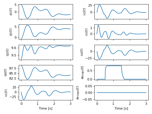
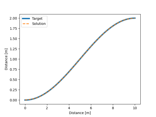
Optimal Bicycle-Rider Trajectories
With all of the above work, we were able to solve an optimal control problem of the muscle-driven bicycle and rider. This is the problem we posed:
Given a multibody model of the Carvallo-Whipple bicycle model extended with a rider that has muscle actuated movable arms and given a desired path on the ground, can we find muscle activations that cause the bicycle-rider to follow the path as closely as possible while minimizing the effort from the representative biceps and triceps?
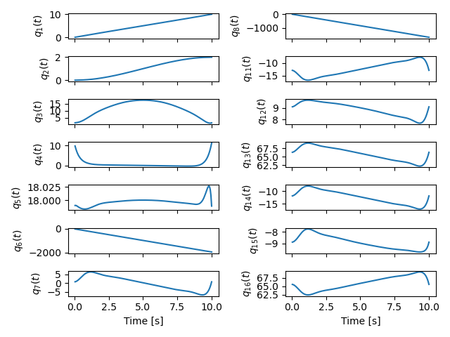
The objective of this optimal control problem takes the form:
where \(x_s\) are a subset of the model's state trajectories and \(x_d\) are some desired trajectories and \(e\) are the muscle excitation inputs. \(w\) is a weighting factor for the two terms. This is a typical minimal effort tracking formulation.
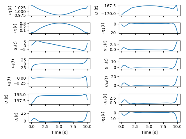
The equations of motion of this system have about 2.8 million mathematical operations. Forming the constraints that represent these equations of motion (a set of differential algebraic equations in this case) involves computing a very large sparse Jacobian with 440 thousand non-zero entries. When we first attempted the differentiation for the Jacobian of the discretized bicycle-rider model, SymPy bogged down on the Jacobian calculation. We let the computation run for over 3 hours and killed the execution before the computation completed. SymPy's differentiation is unusable for interactive work with large equations of motion such as these. Since we already find the common sub-expressions of the equations of motion before code generation in opty, Sam implemented a very efficient forward Jacobian on the expression directed acyclic graph (DAG) in pull request: https://github.com/csu-hmc/opty/pull/102.
This allowed the equations to be differentiated and the differentiation occurs in less than 45 seconds (at least a 250X speed increase), showing the drastic improvements such an approach can have. Once this fix was applied we were finally able to solve the tracking trajectory optimization problem with opty.
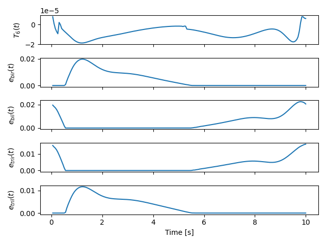
This problem has these characteristics:
- Number of operations in the equations of motion: 2,775,718
- Number of constraints: 6394
- Number of free variables: 7400
- Number of non-zero entries in the Jacobian of the constraints: 439,438
and solves with these timings:
- Time to differentiate the constraints: 43 seconds
- Total time to code generate, form the Jacobian, and compile the C code: 185 seconds
- Average time to evaluate the constraints: 201 µs
- Average time to evaluate the Jacobian: 1.29 ms
- Number of IPOPT iterations: 267
- Time in IPOPT: 45 seconds
 |
 |
 |
 |
The simulation codes and the draft paper about the results can be found in the following repository:
https://github.com/brocksam/muscle-driven-bicycle-paper
The need to evaluate both a function and its Jacobian is a common use case that is not just limited to optimal control problems like the one shown above. SymPy is capable of taking analytical derivatives but it can be prohibitively slow for large expressions. This limits interactive use and rapid iteration in equation derivation. If common sub-expressions are extracted from a SymPy expression, all operations are represented as a directed acyclic graph. Taking the derivative of a DAG instead of a tree graph, as SymPy stores expressions, can provide exponential speedups to differentiation. If the code generation for the function and its Jacobian uses common sub-expression elimination, then it makes sense to call cse() on the function, then take the partial derivatives, and the Jacobian will be in a DAG form for easy code generation. Sam has introduced a major code generation speed up for lambdifying large SymPy expressions if you also desire the Jacobian based on the work we did in opty. The details are in the following pull requests:
Conclusion
We completed almost all of the goals set out in the original proposal along with many more unplanned achievements. SymPy is now more suited for solving non-trivial biomechanical optimal control problems and improvements to the performance of lambdify() will help a broad set of use cases. Our experience also led to many new ideas on how to further improve SymPy for large expression manipulation, especially how unevaluated expression forms that use DAGs as the core data structure can drastically speed up SymPy and reduce the computational resources needed.
Lessons Learned
New contributors to large open source projects should start with pull requests that are small and uncontroversial to build up momentum. Sam started with a pull request to switch SymPy's 15 year old testing framework to pytest. This consumed a lot of time and stalled regularly which in return stalled his other pull requests because he built out the tests with advanced pytest features.
We had planned for 0.5 FTE over the two year period, but it took about 6 months to negotiate a subcontract between TU Delft and Quantsight, since it was the first one of its kind. After that, it took another six months before we interivewed candidates, hired one, and Sam could start. There was not enough time in the grant period for the contract and hiring process. It still worked out, but this is something to plan for in the future.
We developed a large plan for the additions to SymPy that was tough to separate into independent smaller pieces. This led Sam and Timo to work on a set of large interconnected Git branches that would be merged when finished. This ended up leaving us with very large pull requests to review and made it harder for other SymPy developers to interact on the draft work. We also merged all of the new material as private modules (leading underscores in their file names) so that we could make breaking changes in case a SymPy release occurred before we finished the whole plan. The development branch approach was not ideal, SymPy usually has only one development branch, so we should probably avoid that in the future. Merging private modules is a fine approach and is done in other places in SymPy, but you have to have a plan to make them public.
Our proposal had three work packages. After hiring Sam, we realized his prior experience and ideas for SymPy improvement had overlap with Oscar's plans. By the time we understood what exactly we would do, we failed to have more collaborative work between the two related work packages. In the future, it would be good to have more early brainstorm meetings to initiate close collaboration.
Future Plans
We plan to finish any of the unmerged pull requests for the SymPy 1.13 release and the paper on the optimal control of the bicycle-rider system is ongoing work. In the future, we are very interested in incorporating unevaluated expressions and the DAG data structures more into the core of SymPy, as these two ideas can vastly enhance SymPy's performance and the ability to code generate from SymPy expressions with more control and precision. We hope that other users will try out and contribute to the new biomechanics package as well as use SymPy + opty & pycollo for solving optimal control problems of biomechanical multibody systems.
Work Summary
The following list summarizes the various products we have delivered as part of the CZI funding (code, papers, documentation):
- Pull requests to SymPy:
- Pull request to opty: https://github.com/csu-hmc/opty/pull/102
- Pull requests to pycollo:
- Ollie Optimization paper and code:
- BRiM software package:
- Source code: https://github.com/TJStienstra/brim/
- Documentation: https://tjstienstra.github.io/brim/
- BMD 2023 paper: https://doi.org/10.59490/6504c5a765e8118fc7b106c3
- BMD 2023 paper source code: https://github.com/TJStienstra/brim-bmd-2023-paper
- Bicycle steering optimal control paper:
References
| [Meijaard2007] | J. P. Meijaard, J. M. Papadopoulos, A. Ruina, and A. L. Schwab, “Linearized dynamics equations for the balance and steer of a bicycle: A benchmark and review,” Proceedings of the Royal Society A: Mathematical, Physical and Engineering Sciences, vol. 463, no. 2084, pp. 1955–1982, Aug. 2007. |
| [BasuMandal2007] | P. Basu-Mandal, A. Chatterjee, and J. M. Papadopoulos, "Hands-free circular motions of a benchmark bicycle," Proceedings of the Royal Society A: Mathematical, Physical and Engineering Sciences, vol. 463, no. 2084, pp. 1983–2003, Aug. 2007. |
| [DeGroote2016] | De Groote, F., Kinney, A. L., Rao, A. V., & Fregly, B. J., Evaluation of direct collocation optimal control problem formulations for solving the muscle redundancy problem, Annals of biomedical engineering, 44(10), (2016) pp. 2922-2936 |
| [Bird2011] | Richard S. Bird, A simple division-free algorithm for computing determinants, Information Processing Letters, Volume 111, Issues 21–22, 2011, Pages 1072-1074, ISSN 0020-0190, https://doi.org/10.1016/j.ipl.2011.08.006. |