Building Bicycle-Rider Models with SymBRiM

Welcome to this tutorial on creating Symbolic Bicycle-Rider Models using SymBRiM!

In this notebook, we’ll embark on a hands-on journey into SymBRiM, focusing on the practical aspects from a model user’s perspective. By the end of this tutorial, you’ll have achieved the following learning goals:

• Create a Carvallo-Whipple bicycle model using SymBRiM.

• Create a custom bicycle model to suit specific needs.

• Extend a bicycle model to include a rider.

• Parameterize a model using the BicycleParameters library.

• Simulate models using a simple Simulator utility.

• Visualize a model’s behavior with ease using the integrated plotting utility powered by SymMePlot.

Before diving into this tutorial, it’s recommended that you familiarize yourself with the introduction and read through the sections on Software Overview to BRiM Models in the SymBRiM paper. This background information will provide valuable context for what we’ll cover here.

Tutorial Overview

This tutorial is structured as follows: We’ll begin by working with the default Carvallo-Whipple bicycle model, adhering to Moore’s convention. Our journey will encompass configuring the model in SymBRiM, exporting it, and deriving the equations of motion (EoMs). Subsequently, we’ll venture into configuring a new bicycle model, this time incorporating fork suspension. This model will be further extended to include an upper-body rider. Next, we’ll parametrize these models, enabling us to conduct multiple simulations. Finally, we’ll visualize our results as captivating animations.

The Default Bicycle Model

Our starting point is the Carvallo-Whipple bicycle model, following Moore’s convention. The diagram below illustrates the general configuration of this model:

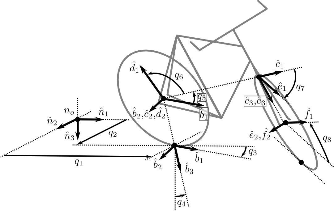
For our initial model, we’ll build the default Carvallo-Whipple bicycle, which aligns perfectly with the image above:

When configuring a bicycle in SymBRiM, each component must be assigned a unique name. Symbol names are derived from component names, so using distinct names is essential. For example, if you would provide "wheel" as the name for both the front wheel and the rear wheel then the symbol for the radius will also be the same symbol. Additionally, SymBRiM applies conventions for certain components. For instance, rear and front frames follow Moore’s convention by default.

Note: You can explicitly specify convention usage by employing ``RigidRearFrame.from_convention(“moore”, “rear_frame”)``.

Exercise: The code below initiates the bicycle configuration. Complete it to match the configuration displayed in the image above.

import warnings

import sympy as sm
import sympy.physics.mechanics as me

import symbrim as sb
from symbrim.bicycle import RigidRearFrameMoore, WhippleBicycleMoore
from symbrim.brim import SideLeanSeatSpringDamper
from symbrim.rider import PinElbowTorque, SphericalShoulderTorque

bicycle_def = sb.WhippleBicycle("my_bike")
assert type(bicycle_def) is WhippleBicycleMoore
bicycle_def.rear_frame = sb.RigidRearFrame.from_convention("moore", "rear_frame")
assert type(bicycle_def.rear_frame) is RigidRearFrameMoore
bicycle_def.rear_wheel = sb.KnifeEdgeWheel("rear_wheel")
bicycle_def.rear_tire = sb.NonHolonomicTire("rear_tire")
### BEGIN SOLUTION
bicycle_def.ground = sb.FlatGround("ground")
bicycle_def.front_frame = sb.RigidFrontFrame("front_frame")
bicycle_def.front_wheel = sb.KnifeEdgeWheel("front_wheel")
bicycle_def.front_tire = sb.NonHolonomicTire("front_tire")
### END SOLUTION
assert len(bicycle_def.submodels) == 5
assert len(bicycle_def.connections) == 2

With the model configured we can now let SymBRiM define the entire model using define_all. This method actually calls five other methods in order, of which the last four were also discussed in the four-bar linkage tutorial:

1. define_connections: All models associate the connections with their required submodels.

2. define_objects: Create the objects, such as symbols reference frames, without defining any relationships between them.

3. define_kinematics: Establish relationships between the objects’ orientations/positions, velocities, and accelerations.

4. define_loads: Specifies the forces and torques acting upon the system.

5. define_constraints: Computes the holonomic and nonholonomic constraints to which the system is subject.

A reason why you may want to call each of these methods manually in order is that you would like to intervene. For example, you may want to change a symbol as done below.

# Manually run all steps
bicycle_def.define_connections()
bicycle_def.define_objects()
display(bicycle_def.rear_wheel.radius, bicycle_def.front_wheel.radius)
# Change the symbol names of the rear and front wheel radius
bicycle_def.rear_wheel.symbols["r"] = sm.Symbol("Rr")
bicycle_def.front_wheel.symbols["r"] = sm.Symbol("Rf")
display(bicycle_def.rear_wheel.radius, bicycle_def.front_wheel.radius)
bicycle_def.define_kinematics()
bicycle_def.define_loads()
bicycle_def.define_constraints()

$\displaystyle rear_{wheel r}$

$\displaystyle front_{wheel r}$

$\displaystyle Rr$

$\displaystyle Rf$

Now we can export this model to a System object from sympy.physics.mechanics.

system_def = bicycle_def.to_system()

At the moment we have not specified any loads, not even gravity. The simplest way to apply gravity is to use System.apply_uniform_gravity. To disturb the bicycle we can apply a lateral force at the saddle, and to control the bicycle a torque actuator at the steer.

Note: loads and constraints can almost always be applied after exporting a model to a system object. The only instance when this is not the case is when the kinematics have to be altered in any way, e.g. using auxiliary speeds.

normal = bicycle_def.ground.get_normal(bicycle_def.ground.origin)
g = sm.symbols("g")
disturbance = me.dynamicsymbols("disturbance")
steer_torque = me.dynamicsymbols("steer_torque")
system_def.apply_uniform_gravity(-g * normal)
system_def.add_loads(
    me.Force(bicycle_def.rear_frame.saddle.point, disturbance * bicycle_def.rear_frame.wheel_hub.axis)
)
system_def.add_actuators(
    me.TorqueActuator(steer_torque, bicycle_def.rear_frame.steer_hub.axis,
                      bicycle_def.rear_frame.steer_hub.frame, bicycle_def.front_frame.steer_hub.frame)
)
system_def.loads, system_def.actuators

((Force(point=rear_frame_wheel_hub_point, force=0),
  Force(point=rear_wheel_masscenter, force=g*rear_wheel_mass*ground_frame.z),
  Force(point=rear_frame_steer_hub_point, force=0),
  Force(point=front_frame_steer_hub_point, force=0),
  Force(point=front_frame_wheel_hub_point, force=0),
  Force(point=front_wheel_masscenter, force=front_wheel_mass*g*ground_frame.z),
  Force(point=ground_origin, force=g*ground_mass*ground_frame.z),
  Force(point=rear_frame_body_masscenter, force=g*rear_frame_body_mass*ground_frame.z),
  Force(point=front_frame_body_masscenter, force=front_frame_body_mass*g*ground_frame.z),
  Force(point=rear_frame_saddle, force=disturbance(t)*rear_frame_body_frame.y)),
 (TorqueActuator(steer_torque(t), axis=rear_frame_body_frame.z, target_frame=rear_frame_body_frame, reaction_frame=front_frame_body_frame),))

Before forming the EoMs we need to specify which generalized coordinates and speeds are independent and which are dependent.

try:
    system_def.validate_system()
except ValueError as e:
    display(e)
system_def.q_ind = [*bicycle_def.q[:4], *bicycle_def.q[5:]]
system_def.q_dep = [bicycle_def.q[4]]
system_def.u_ind = [bicycle_def.u[3], *bicycle_def.u[5:7]]
system_def.u_dep = [*bicycle_def.u[:3], bicycle_def.u[4], bicycle_def.u[7]]
system_def.validate_system()

ValueError('\nThe number of dependent generalized coordinates 0 should be equal to\nthe number of holonomic constraints 1.\n\nThe number of dependent generalized speeds 0 should be equal to the\nnumber of velocity constraints 5.')

Now that everything is define, we can form the EoMs (you can ignore the warnings).

Note: The reason to use ``”CRAMER”`` as constraint solver is to prevent zero-divisions that otherwise occur.

with warnings.catch_warnings():
    warnings.simplefilter("ignore")
    eoms = system_def.form_eoms(constraint_solver="CRAMER")

Congratulations you’ve just created your first bicycle model using SymBRiM!

Modifying a Bicycle

Now that you’ve got a handle on creating a basic bicycle model, let’s start modifying it to include some fork suspension. The best method is to create a new WhippleBicycle object to prevent possible clashes. The model we will use is SuspensionRigidFrontFrame.

Exercise: Complete the configuration of the bicycle model with fork suspension below.

bicycle = sb.WhippleBicycle("bicycle")
### BEGIN SOLUTION
bicycle.ground = sb.FlatGround("ground")
bicycle.rear_wheel = sb.KnifeEdgeWheel("rear_wheel")
bicycle.rear_frame = sb.RigidRearFrame("rear_frame")
bicycle.front_frame = sb.SuspensionRigidFrontFrame("front_frame")
bicycle.front_wheel = sb.KnifeEdgeWheel("front_wheel")
bicycle.rear_tire = sb.NonHolonomicTire("rear_tire")
bicycle.front_tire = sb.NonHolonomicTire("front_tire")
### END SOLUTION
assert len(bicycle.submodels) == 5
assert len(bicycle.connections) == 2
assert isinstance(bicycle.front_frame, sb.SuspensionRigidFrontFrame)

In theory, you could follow the same process now as before and then you will have formed the EoMs of your (first) custom bicycle model. However, we’ll continue by using this bicycle model in a bicycle-rider model.

Extending with a Rider

We can also extend the model with an upper-body rider. We will attach a side-leaning upper-body rider model, where the shoulders are modeled as spherical joints and the elbows as pin joints. To make this extension we create instantiate a bicycle-rider model. This instance we’ll have to provide both our bicycle model, rider model, and the method to connect them. The image below shows the constitution of a complete rider model (not the one we are modeling currently).

Let us start with the rider model.

rider = sb.Rider("rider")
rider.pelvis = sb.PlanarPelvis("pelvis")
rider.torso = sb.PlanarTorso("torso")
rider.left_arm = sb.PinElbowStickLeftArm("left_arm")
rider.right_arm = sb.PinElbowStickRightArm("right_arm")
rider.sacrum = sb.FixedSacrum("sacrum")
rider.left_shoulder = sb.FlexRotLeftShoulder("left_shoulder")
rider.right_shoulder = sb.FlexRotRightShoulder("right_shoulder")

Now let us combine the bicycle and rider models into a single bicycle-rider model. The image below shows the constitution of a complete bicycle-rider model (not the one we are modeling currently). We will just be adding the two models as submodels and the FixedSeat and HolonomicHandGrips connections.

Exercise: Configure the bicycle-rider model accordingly.

bicycle_rider = sb.BicycleRider("bicycle_rider")
### BEGIN SOLUTION
bicycle_rider.bicycle = bicycle
bicycle_rider.rider = rider
bicycle_rider.seat = sb.FixedSeat("seat")
bicycle_rider.hand_grips = sb.HolonomicHandGrips("hand_grips")
### END SOLUTION
assert len(bicycle_rider.submodels) == 2
assert len(bicycle_rider.connections) == 2

To control the bicycle we can make the rider torque-driven by applying torques with the elbows. For this purpose SymBRiM has already dedicated load groups, e.g. PinElbowTorque.

Exercise: Instantiate a load group for each arm with a unique name and assign them to the variables left_arm_lg and right_arm_lg. Next, add each load group to the corresponding arm using add_load_groups.

### BEGIN SOLUTION
left_arm_lg = PinElbowTorque("left_elbow")
rider.left_arm.add_load_groups(left_arm_lg)
right_arm_lg = PinElbowTorque("right_elbow")
rider.right_arm.add_load_groups(right_arm_lg)
### END SOLUTION
assert isinstance(left_arm_lg, PinElbowTorque)
assert isinstance(right_arm_lg, PinElbowTorque)
assert len(rider.left_arm.load_groups) == 1
assert len(rider.right_arm.load_groups) == 1

With the model configured we can let SymBRiM define the model.

Note: to simplify the EoMs we can set the yaw and roll angles of the rider with respect to the rear frame to zero.

bicycle_rider.define_connections()
bicycle_rider.define_objects()
bicycle_rider.seat.symbols["yaw"] = 0
bicycle_rider.seat.symbols["roll"] = 0
bicycle_rider.define_kinematics()
bicycle_rider.define_loads()
bicycle_rider.define_constraints()

Exercise: Export the model to single System instance and assign it to the variable system_br and apply a gravitational and a disturbance force like before.

### BEGIN SOLUTION
system_br = bicycle_rider.to_system()
normal = bicycle_rider.bicycle.ground.get_normal(bicycle_rider.bicycle.ground.origin)
g = sm.symbols("g")
system_br.apply_uniform_gravity(-g * normal)
system_br.add_loads(
    me.Force(bicycle_rider.bicycle.rear_frame.saddle.point,
             disturbance * bicycle_rider.bicycle.rear_frame.wheel_hub.axis)
)
### END SOLUTION
system_br.loads, system_br.actuators

((Force(point=front_frame_suspension_stanchions, force=(-front_frame_c*front_frame_u(t) - front_frame_k*front_frame_q(t))*front_frame_body_frame.z),
  Force(point=front_frame_suspension_lowers, force=(front_frame_c*front_frame_u(t) + front_frame_k*front_frame_q(t))*front_frame_body_frame.z),
  Force(point=rear_frame_body_masscenter, force=g*rear_frame_body_mass*ground_frame.z),
  Force(point=rear_frame_saddle, force=0),
  Force(point=pelvis_masscenter, force=g*pelvis_mass*ground_frame.z),
  Force(point=rear_frame_wheel_hub_point, force=0),
  Force(point=rear_wheel_masscenter, force=g*rear_wheel_mass*ground_frame.z),
  Force(point=rear_frame_steer_hub_point, force=0),
  Force(point=front_frame_steer_hub_point, force=0),
  Force(point=front_frame_wheel_point, force=0),
  Force(point=front_wheel_masscenter, force=front_wheel_mass*g*ground_frame.z),
  Force(point=ground_origin, force=g*ground_mass*ground_frame.z),
  Force(point=front_frame_body_masscenter, force=front_frame_body_mass*g*ground_frame.z),
  Force(point=torso_masscenter, force=g*torso_mass*ground_frame.z),
  Force(point=left_shoulder_int_point, force=0),
  Force(point=left_shoulder_int_point, force=0),
  Force(point=left_arm_upper_arm_masscenter, force=g*left_arm_upper_arm_mass*ground_frame.z),
  Force(point=right_shoulder_int_point, force=0),
  Force(point=right_shoulder_int_point, force=0),
  Force(point=right_arm_upper_arm_masscenter, force=g*right_arm_upper_arm_mass*ground_frame.z),
  Force(point=left_arm_forearm_masscenter, force=g*left_arm_forearm_mass*ground_frame.z),
  Force(point=right_arm_forearm_masscenter, force=g*right_arm_forearm_mass*ground_frame.z),
  Force(point=rear_frame_saddle, force=disturbance(t)*rear_frame_body_frame.y)),
 (TorqueActuator(left_elbow_T(t), axis=left_arm_upper_arm_frame.y, target_frame=left_arm_forearm_frame, reaction_frame=left_arm_upper_arm_frame),
  TorqueActuator(right_elbow_T(t), axis=right_arm_upper_arm_frame.y, target_frame=right_arm_forearm_frame, reaction_frame=right_arm_upper_arm_frame)))

Exercise: Set the independent and dependent generalized coordinates and speeds of system_br.

Hint: You can use the same division for ``bicycle_rider.bicycle.q`` and ``bicycle_rider.bicycle.u`` as before for ``bicycle_def``.

### BEGIN SOLUTION
b, r = bicycle_rider.bicycle, bicycle_rider.rider
system_br.q_ind = [
    *b.q[:4], *b.q[5:], *b.front_frame.q
]
system_br.q_dep = [
    b.q[4], *r.left_shoulder.q, *r.right_shoulder.q, *r.left_arm.q, *r.right_arm.q
]
system_br.u_ind = [
    b.u[3], *b.u[5:7], *b.front_frame.u
]
system_br.u_dep = [
    *b.u[:3], b.u[4], b.u[7], *r.left_shoulder.u, *r.right_shoulder.u, *r.left_arm.u, *r.right_arm.u
]
### END SOLUTION
system_br.validate_system()

Exercise: Form the equations of motion and use "CRAMER" as constraint solver.

### BEGIN SOLUTION
with warnings.catch_warnings():
    warnings.simplefilter("ignore")
    eoms = system_br.form_eoms(constraint_solver="CRAMER")
### END SOLUTION
assert system_br.mass_matrix

Congratulations! You have just built your (first) bicycle-rider model.

Parametrization

While it is possible to manually figure out all parameters and create a dictionary to map all symbols accordingly, SymBRiM integrates support for the BicycleParameters package. The BicycleParameters package is designed to generate, manipulate, and visualize the parameters of the Whipple-Carvallo bicycle model. The repository provides several measured parametrizations. For instructions on measuring your own bicycle and/or rider refer to Moore’s dissertation.

The code below imports the parametrization library and instantiates a parametrization object, which loads in "Jason" on the Batavus "Browser" bicycle.

Note: This cell will download some parametrization data if it is not already present.

from pathlib import Path

import bicycleparameters as bp
import numpy as np
from utils import download_parametrization_data

data_dir = Path.cwd() / "data"
if not data_dir.exists():
    download_parametrization_data(data_dir)
bike_params = bp.Bicycle("Browser", pathToData=data_dir)
bike_params.add_rider("Jason", reCalc=True)

Found the RawData directory: /home/runner/work/symbrim/symbrim/docs/tutorials/data/bicycles/Browser/RawData
Looks like you've already got some parameters for Browser, use forceRawCalc to recalculate.
There is no rider on the bicycle, now adding Jason.
Calculating the human configuration.

To get a mapping of symbols to values based on this parametrization we can use get_param_values as shown below.

constants_def = bicycle_def.get_param_values(bike_params)
constants_def[g] = 9.81  # Don't forget to specify the gravitational constant.
constants_def

{rear_frame_body_mass: 9.86,
 rear_frame_l_bbx: np.float64(0.40374135119327337),
 rear_frame_l_bbz: np.float64(0.22043802153129097),
 rear_frame_ixx: 0.6473909751608555,
 rear_frame_iyy: 1.3163960124977576,
 rear_frame_izz: 0.6390248264511185,
 rear_frame_izx: -0.16249625380874022,
 rear_frame_d1: 0.963149263487593,
 rear_frame_l1: 0.3308144077188117,
 rear_frame_l2: -0.07398701275972652,
 rear_frame_d4: np.float64(0.4225541286665965),
 rear_frame_d5: np.float64(-0.5493321255935064),
 front_frame_body_mass: 3.22,
 front_frame_ixx: 0.28109686661693817,
 front_frame_iyy: 0.245827908036,
 front_frame_izz: 0.06782716361036183,
 front_frame_izx: 0.00634846730073884,
 front_frame_d2: 0.4338396131640938,
 front_frame_d3: 0.0705000000001252,
 front_frame_l3: -0.07654646159268344,
 front_frame_l4: -0.47166687226492093,
 front_frame_d6: np.float64(-0.17310563866173195),
 front_frame_d7: np.float64(0.29),
 front_frame_d8: np.float64(-0.37486632400446973),
 rear_wheel_mass: 3.11,
 rear_wheel_ixx: 0.0904114316323,
 rear_wheel_iyy: 0.152391250767,
 Rr: 0.340958858855,
 front_wheel_mass: 2.02,
 front_wheel_ixx: 0.0883826870796,
 front_wheel_iyy: 0.149221207336,
 Rf: 0.34352982332,
 g: 9.81}

The code below defines a function to quickly retrieve all symbols defined in a model. Next, we obtain all symbols defined in the bicycle models and if there are still symbols missing in our constants_def dictionary.

missing_symbols = bicycle_def.get_all_symbols().difference(constants_def.keys())
missing_symbols

set()

Exercise: Create a constants_br dictionary for the bicycle_rider model and obtain the missing symbols (missing_symbols).

Note: you may use the same parametrization ``bike_params`` as before.

### BEGIN SOLUTION
constants_br = bicycle_rider.get_param_values(bike_params)
missing_symbols = bicycle_rider.get_all_symbols().difference(constants_br.keys())
### END SOLUTION
assert len(constants_br) >= 87
missing_symbols

{front_frame_c,
 front_frame_d9,
 front_frame_k,
 left_elbow_T(t),
 right_elbow_T(t),
 seat_pitch}

To quickly see what this symbol is used for we can ask the model to get a description for each:

for sym in missing_symbols:
    display(f"{sym} - {bicycle_rider.get_description(sym)}")

'front_frame_k - Spring stiffness of the front suspension.'

'front_frame_d9 - Perpendicular distance from the steer axis to the suspension.'

'seat_pitch - Pitch angle of the pelvis w.r.t. the rear frame.'

'left_elbow_T(t) - Elbow torque of left_arm'

'right_elbow_T(t) - Elbow torque of right_arm'

'front_frame_c - Damping coefficient of the front suspension.'

As these symbols have not been defined by the bicycle parameters data we need to define them manually. However, some of them are inputs, so those we’ll specify later on.

constants_br.update({
    bicycle_rider.bicycle.front_frame.symbols["d9"]: constants_br[bicycle_rider.bicycle.front_frame.symbols["d3"]],
    bicycle_rider.bicycle.front_frame.symbols["k"]: 19.4E3,
    bicycle_rider.bicycle.front_frame.symbols["c"]: 9E3,
    bicycle_rider.seat.symbols["pitch"]: -0.7,
    g: 9.81  # Just in case you did not specify the gravitational constant yet.
})

Warning: Above we do forget to take into account the inertia and mass of the legs. A good option would have been computing their contribution and adding that to the rear frame’s mass and inertia.

Simulation Bicycle Model

Now that we have a parametrized model we can simulate it. SymBRiM does not provide a simulation utility (yet), but a separate module has here been provided implementing a simple simulation utility. The code below imports this utility and initializes a simulation object for the bicycle model.

import numpy as np
from simulator import Simulator

sim_def = Simulator(system_def)

Before running the actual simulation we need to specify three things: - constants: A dictionary mapping static symbols to values. - initial_conditions: A dictionary mapping generalized coordinates and speeds to initial values. - inputs: A dictionary mapping input symbols to a function taking the time and state as arguments, i.e. f(t, x) -> float.

The code below sets each of these for the bicycle model, where an initial guess for the rear frame pitch is provided and the rear wheel is given an initial angular velocity. The disturbance inputs is a sine wave that increases in amplitude over time. For the steer input, we’ll use a simple proportional controller that applies a torque proportional to the roll rate to stabilize the bicycle.

sim_def.constants = constants_def
sim_def.initial_conditions = {
    **{xi: 0.0 for xi in system_def.q.col_join(system_def.u)},
    bicycle_def.q[4]: 0.314,  # Initial guess rear frame pitch.
    bicycle_def.u[5]: -3.0 / constants_def[bicycle_def.rear_wheel.radius],  # Rear wheel angular velocity.
}
roll_rate_idx = len(system_def.q) + system_def.u[:].index(bicycle_def.u[3])
max_roll_rate, max_torque = 0.2, 10
sim_def.inputs = {
    disturbance: lambda t, x: (30 + 30 * t) * np.sin(t * 2 * np.pi),
    steer_torque: lambda t, x: -max_torque * max(-1, min(x[roll_rate_idx] / max_roll_rate, 1)),
}

Now we can initialize the simulator objects, which automatically solves the initial conditions for us.

Note: the initialization of a simulator object can take a while, so be patient.

sim_def.initialize()
sim_def.initial_conditions

{my_bike_q1(t): 0.0,
 my_bike_q2(t): 0.0,
 my_bike_q3(t): 0.0,
 my_bike_q4(t): 0.0,
 my_bike_q6(t): 0.0,
 my_bike_q7(t): 0.0,
 my_bike_q8(t): 0.0,
 my_bike_q5(t): np.float64(0.399680398706867),
 my_bike_u4(t): 0.0,
 my_bike_u6(t): -8.79871551094032,
 my_bike_u7(t): 0.0,
 my_bike_u1(t): np.float64(2.9999999999999996),
 my_bike_u2(t): np.float64(-1.7142933546584113e-28),
 my_bike_u3(t): np.float64(3.057822083862947e-28),
 my_bike_u5(t): np.float64(-1.2576551361634348e-16),
 my_bike_u8(t): np.float64(-8.732866250175556)}

With the simulator initialized we can run the simulation. The code below runs the simulation for 2.5 seconds. A DAE solver is used with a relative tolerance of 1e-3 and an absolute tolerance of 1e-6.

sim_def.solve(np.arange(0, 2.5, 0.01), solver="dae", rtol=1e-3, atol=1e-6)
sim_def.t[-1]

np.float64(2.49)

Visualizing the Bicycle Simulation Results

Using the Plotter from SymBRiM we can easily visualize the model and create an animation based on the simulation results.

import matplotlib.pyplot as plt
from IPython.display import HTML
from matplotlib.animation import FuncAnimation
from scipy.interpolate import CubicSpline

from symbrim.utilities.plotting import Plotter

# Create some functions to interpolate the results.
x_eval = CubicSpline(sim_def.t, sim_def.x.T)
r_eval = CubicSpline(sim_def.t, [[cf(t, x) for cf in sim_def.inputs.values()]
                                 for t, x in zip(sim_def.t, sim_def.x.T)])
p, p_vals = zip(*sim_def.constants.items())
max_disturbance = r_eval(sim_def.t)[:, tuple(sim_def.inputs.keys()).index(disturbance)].max()

# Plot the initial configuration of the model
fig, ax = plt.subplots(subplot_kw={"projection": "3d"}, figsize=(8, 8))
plotter = Plotter.from_model(bicycle_def, ax=ax)
plotter.add_vector(disturbance * bicycle_def.rear_frame.wheel_hub.axis / max_disturbance,
                   bicycle_def.rear_frame.saddle.point, name="disturbance", color="r")
plotter.lambdify_system((system_def.q[:] + system_def.u[:], sim_def.inputs.keys(), p))
plotter.evaluate_system(x_eval(0.0), r_eval(0.0), p_vals)
plotter.plot()
X, Y = np.meshgrid(np.arange(-1, 10, 0.5), np.arange(-1, 3, 0.5))
ax.plot_wireframe(X, Y, np.zeros_like(X), color="k", alpha=0.3, rstride=1, cstride=1)
ax.invert_zaxis()
ax.invert_yaxis()
ax.set_xlim(X.min(), X.max())
ax.set_ylim(Y.min(), Y.max())
ax.view_init(19, 14)
ax.set_aspect("equal")
ax.axis("off")

fps = 30
ani = plotter.animate(
    lambda ti: (x_eval(ti), r_eval(ti), p_vals),
    frames=np.arange(0, sim_def.t[-1], 1 / fps),
    blit=False)
display(HTML(ani.to_jshtml(fps=fps)))
plt.close()

Once Loop Reflect

Simulating the Bicycle-Rider Model

Now that we know how to simulate the bicycle model, we can perform a similar simulation for the bicycle-rider model we have created.

Exercise: Initiate a simulator object for the bicycle-rider model and assign in to sim_br.

### BEGIN SOLUTION
sim_br = Simulator(system_br)
### END SOLUTION
assert sim_br.system is system_br

Exercise: Set the constants, initial conditions, and inputs of sim_br. For the inputs try using a similar control for the elbow torques as before for the steer torque.

Hint: You can access the torques of the load groups from their ``symbols`` dictionary, e.g. ``left_arm_lg.symbols[“T”]``.

### BEGIN SOLUTION
sim_br.constants = constants_br
sim_br.initial_conditions = {
    **{xi: 0.0 for xi in system_br.q.col_join(system_br.u)},
    bicycle_rider.bicycle.q[4]: 0.314,  # Initial guess rear frame pitch.
    bicycle_rider.bicycle.u[5]: -3.0 / constants_br[bicycle_rider.bicycle.rear_wheel.radius],
    bicycle_rider.rider.left_arm.q[0]: 0.7,  # Elbow flexion.
    bicycle_rider.rider.right_arm.q[0]: 0.7,  # Elbow flexion.
    bicycle_rider.rider.left_shoulder.q[0]: 0.5,  # Shoulder flexion.
    bicycle_rider.rider.right_shoulder.q[0]: 0.5,  # Shoulder flexion.
    bicycle_rider.rider.left_shoulder.q[1]: -0.6,  # Shoulder rotation.
    bicycle_rider.rider.left_shoulder.q[1]: -0.6,  # Shoulder rotation.
    bicycle_rider.bicycle.u[3]: 0.3,
}
roll_idx = system_br.q[:].index(bicycle_rider.bicycle.q[3])
roll_rate_idx = len(system_br.q) + system_br.u[:].index(bicycle_rider.bicycle.u[3])
max_roll_rate, max_torque = 0.2, 10
bound = lambda x: max(-1, min(x, 1))
excitation = lambda x:  bound(x[roll_rate_idx] / max_roll_rate)

sim_br.inputs = {
    disturbance: lambda t, x: (30 + 30 * t) * np.sin(t * 2 * np.pi),
    left_arm_lg.symbols["T"]: lambda t, x: -max_torque * excitation(x),
    right_arm_lg.symbols["T"]: lambda t, x: max_torque * excitation(x),
}
### END SOLUTION
assert len(sim_br.constants) == 92
assert len(sim_br.initial_conditions) == 30
assert len(sim_br.inputs) == 3

Exercise: Initialize the simulator.

Hint: If a runtime error from scipy.fsolve is shown, then it was not able to solve the initial conditions. Recommendable is to update your initial conditions to provide a better guess and use ``sim_br.solve_initial_conditions()`` without reinitializing the simulator object.

Note: Initializing the bicycle-rider simulator takes longer than initializing just the bicycle.

### BEGIN SOLUTION
sim_br.initialize()
### END SOLUTION
sim_br.eval_rhs(0, [sim_br.initial_conditions[xi] for xi in system_br.q[:] + system_br.u[:]])

array([ 3.00000000e+00,  3.26841150e-33, -5.69472114e-16,  3.00000000e-01,
       -8.79871551e+00, -0.00000000e+00, -8.73286625e+00,  0.00000000e+00,
       -0.00000000e+00,  1.56914295e-27, -2.22877858e-28,  1.39570538e-27,
       -4.37780608e-27, -3.28954997e-28, -1.15750563e-27, -1.75919306e-01,
        2.42600844e+01,  1.40657668e+01,  9.59312566e+00, -5.58384985e+00,
       -1.55431223e-15,  7.92697958e-01, -7.88318230e+00,  3.49448718e+01,
        1.44833210e+01, -1.93488172e+01, -1.44833210e+01,  1.93488172e+01,
       -7.45538540e+00,  7.45538540e+00])

Exercise: Peform a simulation over a time-span of 2.5 seconds using a DAE solver.

Hint: If the simulation fails it can be that the controls are unstable causing the bicycle to fall or that something else is wrong. A simple solution is to use an ODE integrator to figure out the controls: ``sim_br.solve((0, 2.5), t_eval=np.arange(0, 2.5, 0.01))``. Also, feel free to reduce the disturbance force to make the control easier.

### BEGIN SOLUTION
# sim_br.solve(np.arange(0, 2.5, 0.01), solver="dae", rtol=1e-3, atol=1e-6)
sim_br.solve((0, 2.5), t_eval=np.arange(0, 2.5, 0.01))
### END SOLUTION
sim_br.t[-1]

np.float64(2.49)

Visualizing the Bicycle-Rider Simulation

The simulation can be visualized using similar code as below.

Exercise: Complete the code below by initializing the Plotter, optionally adding a vector for the disturbance, and running lambdify_system.

# Create some functions to interpolate the results.
x_eval = CubicSpline(sim_br.t, sim_br.x.T)
r_eval = CubicSpline(sim_br.t, [[cf(t, x) for cf in sim_br.inputs.values()]
                                 for t, x in zip(sim_br.t, sim_br.x.T)])
p, p_vals = zip(*sim_br.constants.items())
max_disturbance = r_eval(sim_br.t)[:, tuple(sim_br.inputs.keys()).index(disturbance)].max()

# Plot the initial configuration of the model
fig, ax = plt.subplots(subplot_kw={"projection": "3d"}, figsize=(8, 8))
### BEGIN SOLUTION
plotter = Plotter.from_model(bicycle_rider, ax=ax)
plotter.add_vector(disturbance * bicycle_rider.bicycle.rear_frame.wheel_hub.axis / max_disturbance,
                   bicycle_rider.bicycle.rear_frame.saddle.point, name="disturbance", color="r")
plotter.lambdify_system((system_br.q[:] + system_br.u[:], sim_br.inputs.keys(), p))
### END SOLUTION
plotter.evaluate_system(x_eval(0.0), r_eval(0.0), p_vals)
plotter.plot()
X, Y = np.meshgrid(np.arange(-1, 10, 0.5), np.arange(-1, 4, 0.5))
ax.plot_wireframe(X, Y, np.zeros_like(X), color="k", alpha=0.3, rstride=1, cstride=1)
ax.invert_zaxis()
ax.invert_yaxis()
ax.set_xlim(X.min(), X.max())
ax.set_ylim(Y.min(), Y.max())
ax.view_init(19, 14)
ax.set_aspect("equal")
ax.axis("off")

fps = 30
ani = plotter.animate(
    lambda ti: (x_eval(ti), r_eval(ti), p_vals),
    frames=np.arange(0, sim_br.t[-1], 1 / fps),
    blit=False)
display(HTML(ani.to_jshtml(fps=fps)))
plt.close()

Once Loop Reflect

Congratulations! You have completed this tutorial.